Tutorial
In this chapter, the implementation of each module in MODAS will be introduced in detail, and several real-data results will also be shown in order to help users understand the principles of MODAS in depth. Moreover, a reference pipeline is also provided to help users analyze their own data. The datasets used in this part include a genotype data and a kernel metabolome data from a maize AMP population of 510 inbred lines.
Genotype dimensionality reduction analysis
Necessity and algorithms of genotype dimensionality reduction
Genome-wide association analysis (GWAS) is a common method for identifying quantitative trait loci (QTL). With the rapid development of transcriptome, metabolomics and other high-throughput omics technologies, multi-omics data is gradually used as molecular traits (mTraits) for GWAS analysis. However, GWAS is generally used to analyze a small number of phenotypic traits. In terms of high-dimensional omics data molecular traits, conventional GWAS method is faced with such problems as large computational resource consumption, redundant data and difficult interpretation of analytical results. Generally, the high-dimensional molecular traits datasets include thousands of points, while the genotype datasets include millions of data points. Thus, a key step of association analysis for high-dimensional omics data is to reduce the dimensionality of the data. Due to linkage disequilibrium (LD), there are highly linked SNPs in a population's genotype file, which are highly redundant. We can use dimensionality reduction method to generate a pseudo-genotype file from the original SNP-based genotype file, which can dramatically reduce the dimensionality of genotype data, and improve the efficiency of GWAS to identifying QTLs quickly.
In MODAS, Jaccard similarity coefficient, DBSCAN and PCA algorithms are jointly used for dimensionality reduction of SNP-base genotype data. In general, major allele accounts for a small proportion of heritability, while minor allele is more likely to be risk allele, therefore, the measurement of minor allele similarity can better reflect the functional similarity of SNP loci. In detail, given two SNP loci SNP1 and SNP2, use A to represent the number of minor alleles in all samples for SNP1, and use B to represent the number of minor alleles in all samples for SNP2, then, the ratio of the intersection size of A to B to the size of the union of A and B is defined as Jaccard similarity coefficient J(A,B). The larger J(A,B) value is, the higher the sample similarity is, when both A and B are empty, J(A,B) is defined as zero. Since DBSCAN is a density-based clustering algorithm, it defines the largest set of densely-connected points as clusters, clustering patterns of arbitrary shapes can be found in high-noise spaces. Compared with distance-based clustering algorithms such as K-means, DBSCAN does not need to know the number of clusters in advance, and can find clusters of any shape, as well as remove noise points. While compared with linkage disequilibrium based haplotype and tag SNP method, DBSCAN as a kind of non-supervised machine learning method, can better persist the genotype characteristic of genomic blocks, does not rely on biological parameters and has speed advantage. In addition, as a commonly used linear dimension reduction method, PCA has advantages in speed and accuracy. Thus, to sum up the advantages of these algorithms, Jaccard similarity coefficient distance matrix of minor alleles is used as the input of DBSCAN cluster algorithm to generate genomic blocks, and PCA is used for extract pseudo-genotypes from genomic blocks.
Feasibility of genotype dimensionality reduction
Here, we take a known QTL of metabolite DFP (Wen et al.) as an example to exhibit the feasibility of performing association analysis using pseudo-genotypes generated by dimensionality reduction as input. First, we performed SNP-based GWAS on DFP and get a QTL region between 142MB and 143.5MB on chromosome 1. The Manhattan plot is as follow:

Then, we extracted the SNPs in this genomic region, and calculated the similarity coefficients of pairwise SNPs in the region through the Jaccard similarity coefficient, and then clustered the SNPs in the region through DBSCAN algorithm. The clustering result is as follow:
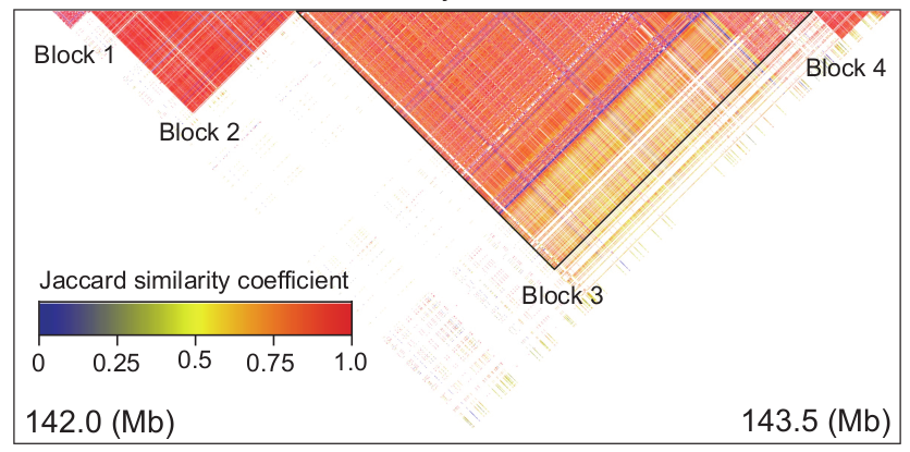
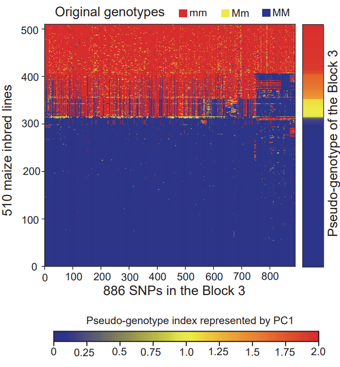
It can be seen from the figure that there are mainly 4 highly linked blocks in the QTL of DFP. Among them, block3 is significantly related to the content of DFP. Principal component analysis of block3 shows that the first principal component of block3 can represent the genotype difference of all SNPs in block3. Therefore, it is feasible to perform dimensionality reduction analysis on the SNP-based genotypes to generate pseudo-genotypes for association analysis. The SNP-based genotype difference of block3 and the first principal component difference after dimensionality reduction are shown in the figure below.
Generate genome wide pseudo-genotype files
PCA as a dimensionality reduction method for genome-wide genotype data has been widely used in population structure analysis, but it can only reflect the genetic difference on the whole genome level, while the principle of QTL identification is based on specific genomic region difference among individuals in a population. However, segmentation of the whole genome may lead a result that same linkage genomic regions be assigned to different windows, which would reduce the power of association analysis. In order to prevent this situation, a sliding window method is implemented in MODAS to perform dimensionality reduction analysis on the whole genome scale. The parameter for generating genome-wide pseudo-genotype files is -genome_cluster, the parameter for setting the window size is -w, with the default value 1Mb, and the parameter for setting the step size is -s, with the default value 0.5Mb.
The command line is as follows:
# default window and step
MODAS genoidx -g ./chr_HAMP -genome_cluster -p 10 -o chr_HAMP

# set window 2MB
MODAS genoidx -g ./chr_HAMP -genome_cluster -w 2000000 -p 10 -o chr_HAMP

# set window 2MB step 1MB
MODAS genoidx -g ./chr_HAMP -genome_cluster -w 2000000 -s 1000000 -p 10 -o chr_HAMP
In the above command lines, -p specifies the number of chromosomes for dimensionality reduction analysis simultaneously, and the maximum is the number of chromosomes in the dimensionality reduction analysis; -g specifies the plink-bed format genotype file for dimensionality reduction analysis; -o specifies the prefix of the output file. The suffix of the generated output pseudo-genotype files are genome_cluster.csv.
Convert hapmap format to plink-bed format
The input genotype file of MODAS is plink-bed format. Since the hapmap format is also commonly used, MODAS implements a function of converting the hapmap format to plink-bed format. This can be called by the parameter -convert.
The command line is as follows:
# convert hapmap genotype file to plink bed genotype file
MODAS genoidx -g ./chr_HAMP.hap -convert -o ./chr_HAMP

# convert hamap genotype file and generate pseudo-genotype file
MODAS genoidx -g ./chr_HAMP.hap -convert -genome_cluster -p 10 -o ./chr_HAMP
Generate pseudo-genotype files for a large number of SNPs (~10 million)
When generating pseudo-genotype files for a particularly large number of SNPs (~10 million), it would be very slow. In order to solve this problem, MODAS introduces clumping analysis to retain SNPs that are almost unrelated to each other. In this way, it can not only reduce the size of the genotype file, but also retain the diversity of the population without affecting the subsequent association analysis. This SNP clumping analysis can be called by the parameter -clump.
The command line is as follows:
# clumping analysis
MODAS genoidx -g ./chr_HAMP -clump -o ./chr_HAMP

# clumping analysis and generate pseudo-genotype file
MODAS genoidx -g ./chr_HAMP -clump -genome_cluster -p 10 -o ./chr_HAMP
The clumping analysis will generate genotype files in plink-bed format with suffixes _clump.bed, _clump.bim, and _clump.fam.
Phenotype preprocessing and transformation
Filter the phenotype data
Phenotype data with high missing rates and low values may reduce the accuracy of association analysis. Two parameters -r and -v can be used to filter the phenotype data based on missing rates and phenotype values, respectively. MODAS considers both NA and 0 to be missing data when calculates missing rates. MODAS filters phenotype values by this criterion: the phenotype whose average value is higher than the threshold is retained, while the phenotype value below this threshold is dropped.
The command line is as follows:
# filter missing rate 0.5
MODAS phenorm -phe phe_data.csv -r 0.5 -o phe_data

# filter value lower than 1
MODAS phenorm -phe phe_data.csv -v 1 -o phe_data

# filter missing rate 0.5 and value lower than 1
MODAS phenorm -phe phe_data.csv -r 0.5 -v 1 -o phe_data
Transform the phenotype data
Omics data generally differ by orders of magnitude and population sturcture, which would lead to inaccurate association analysis results. MODAS supports logarithmization and normalization of the phenotype data to reduce the order of magnitude differences, correct the differences in phenotype caused by population structure through PCA. Different degrees of logarithmization can be performed by calling the parameters -log2, -ln, and -log10. The box-cox method can be used to normalize the phenotype data by calling the parameter -norm, The normal quantile method can be used to normalize the phenotype data by calling the parameter -qqnorm. Correct the differences caused by population structure can by performed by calling the parameters -pca, the genotype file for calculating PCA is specified by parameter -g.
The command line is as follows:
# log2 transformation
MODAS phenorm -phe phe_data.csv -log2 -o phe_data

# normal distribution transformation
MODAS phenorm -phe phe_data.csv -norm -o phe_data

# normal quantile transformation
MODAS phenorm -phe phe_data.csv -qqnorm -o phe_data

# correct phenotype by PCA and normal quantile transformation
MODAS phenorm -phe AMP_kernel_transcriptome_v4_FPKM.csv -g chr_HAMP -pca -qqnorm -o AMP_kernel_transcriptome_v4_FPKM_correct
The suffix of the generated normalized phenotype data file is normalized_phe.csv.
Prescreen candidate genomic regions
When using pseudo-genotype files to perform association analysis on high-dimensional omics data, we provide three models of LM (implemented in GEMMA), GLM (implemented in rMVP) and MLM (implemented in GEMMA) so that the association analysis is suitable for different types of omics phenotypes. Then, MODAS screened genomic blocks using a significance threshold(default is 1 divided by the number of blocks) to obtain the candidate significantly associated genomic regions.
This step can be accomplished by the subcommand prescreen in MODAS. Two files with suffixes phe_sig_qtl.csv and sig_omics_phe.csv will be generated, corresponding to the candidate genomic regions and candidate molecular traits, respectively. The prescreen step also need a kinship matrix as input which can be calculated automatically based on the SNP-based genotype file, which is specified by the parameter -g. The -gwas_suggest_pvalue parameter is used to specify the significance threshold of gwas model, the -gwas_model parameter specifies model used in pseudo-genotype association analysis, and the -genome_cluster parameter specifies the pseudo-genotype files.
The command line is as follows:
# prescreening candidate QTLs with default parameters
MODAS prescreen -g ./chr_HAMP -genome_cluster ./chr_HAMP.genome_cluster.csv -phe ./E3_log2.normalized_phe.csv -o E3_log2

# perscreening candidate QTLs with 20 threads, specifies by -p
MODAS prescreen -g ./chr_HAMP -genome_cluster ./chr_HAMP.genome_cluster.csv -phe ./E3_log2.normalized_phe.csv -p 20 -o E3_log2

# set the threshold of GWAS P value to 1e-5, and the GWAS model is MLM
MODAS prescreen -g ./chr_HAMP -genome_cluster ./chr_HAMP.genome_cluster.csv -phe ./E3_log2.normalized_phe.csv -p 20 -gwas_suggest_pvalue 1e-5 -gwas_model MLM -o E3_log2
Perform regional association analysis to identify QTLs
Perform regional association analysis on candidate genomic regions
Through the prescreen of pseudo-genotype files, the candidate genomic regions can be obtained, but the accurate boundaries of the QTLs still cannot be obtained. In order to accurately obtain the boundary for each QTL, MODAS performs SNP-based regional association analysis using LM (implemented in GEMMA), GLM (implemented in rMVP), or MLM (implemented in GEMMA) on these candidate genomic regions, and uses plink clumping analysis to merge the linked (R2=0.2) significant SNPs, to determine the precise boundaries of each QTL. Finally, a QTL with more than 10 SNPs is regarded as a reliable QTL. Since the SNPs in a QTL region cannot accurately reflect the genetic relationship of inbred lines, a SNP-based genotype file is also needed through the parameter -g for kinship matrix calculation.
The command line is as follows:
# identify QTLs with default parameters
MODAS regiongwas -g ./chr_HAMP -phe ./E3_log2.sig_omics_phe.csv -phe_sig_qtl ./E3_log2.phe_sig_qtl.csv -o E3_log2

# identify QTLs with 20 threads, specifies by -p
MODAS regiongwas -g ./chr_HAMP -phe ./E3_log2.sig_omics_phe.csv -phe_sig_qtl ./E3_log2.phe_sig_qtl.csv -p 20 -o E3_log2

# identify QTLs with p1 = 1e-7 and p2 = 1e-6
MODAS regiongwas -g ./chr_HAMP -phe ./E3_log2.sig_omics_phe.csv -phe_sig_qtl ./E3_log2.phe_sig_qtl.csv -p1 1e-7 -p2 1e-6 -p 20 -o E3_log2

# identify QTLs with GLM model
MODAS.py regiongwas -g ./chr_HAMP -phe ./E3_log2.sig_omics_phe.csv -phe_sig_qtl ./E3_log2.phe_sig_qtl.csv -gwas_modle GLM -p 20 -o E3_log2
The -phe_sig_qtl parameter specifies the candidate genomic regions file, the -phe parameter specifies the candidate traits file, the -g parameter specifies the SNP-based genotype file, the -p1 parameter specifies the significance threshold of index SNPs, the -p2 parameter specifies the secondary significance threshold for clumped SNPs, the -gwas_model parameter specifies gwas model used in regionnal association analysis. The regiongwas subcommand generates two files with the suffixes local_gwas_qtl_res.csv and local_gwas_bad_qtl_res.csv, which deposit reliable QTLs and unreliable QTLs, respectively.
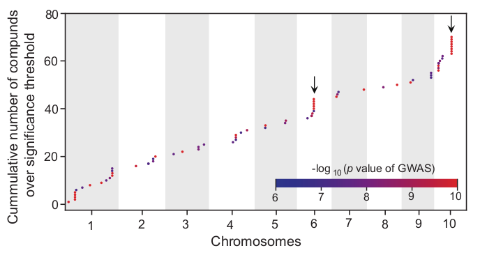
The cumulative distribution of significantly associated QTLs/metabolites after regional association analysis is looks like this:
Cluster the molecular traits
In the results of regional association analysis, the QTLs identified by different traits were sometimes overlapped. Principal component analysis can be performed for the traits with overlapped QTLs, and the first principal component PC1 be used for GWAS analysis. As a result, the same QTL could be detected, which indicated that PC1 could replace the original multiple traits to reduce the amount of computing resource. In the process of regional association analysis in MODAS, the -cluster parameter can be added to cluster the traits according to the distance between QTL positions and further reduce the dimension of the molecular traits.
In detail, the steps are as follows: First, when peak SNPs for two traits with a distance less than 2Mb, these traits are clustered. Second, principal component analysis is performed on the cluster and the correlation between the first principal component (PC1) and each trait are calculated. Third, when all traits have correlations greater than 0.6 with PC1 and the number of traits are greater than 2, these traits are clustered; whilst the remaining traits with correlations smaller than 0.6 are subjected to a new round a PCA; then, repeat the steps above until there is no trait remaining or no trait has a correlation greater than 0.6 with PC1, the remaining phenotypes are output separately.
The command line is as follows:
# identify QTLs with 20 threads and cluster molecular traits
MODAS.py regiongwas -g ./chr_HAMP -phe ./E3_log2.sig_omics_phe.csv -phe_sig_qtl ./E3_log2.phe_sig_qtl.csv -p 20 -cluster -o E3_log2
-cluster parameter will generate two files with the suffixes phe_labeled.csv and clustered_phe.csv, which correspond to the cluster label of each traits and the reduced-dimensional traits, respectively.
Perform Mendelian randomization analysis
Mendelian Randomization analysis
Mendelian Randomization (MR) has been successfully applied in human genetics to explain the causal relations among genetic mutations, intermediate phenotypes (e.g., hypertension, hyperlipidemia) and diseases (e.g., stroke, myocardial infarction), rather than only associations. MODAS uses two models for Mendelian randomization analysis. In linear model, z represents the most significantly associated SNP of mTrait detected in RA analysis, x represents the expression level of a mTrait, and y represents the pTrait. Then, a two-step least-squares (2SLS) estimate of the effect of x on y from an MR analysis is:

where bzy and bzx are the least-squares estimates of z on y and x, respectively, and bxy is interpreted as the effect size of x on y free of confounding from non-genetic factors. The sampling variance of the 2SLS estimate is:

where n is the sample size,\(R_{xy}^2\) is the proportion of variance in y explained by x, and \(R_{zx}^2\) is the proportion of variance in x explained by z. In mixed linear model, z represents the most significantly associated SNP of mTrait detected in RA analysis, bzy is the estimate of the most significantly associated SNP effect from mixed linear model for pTrait, var(bzy) is the estimate of the most significantly associated SNP standard error from mixed linear model for pTrait, bzx is the estimate of the most significantly associated SNP effect from mixed linear model for mTrait, var(bzx) is the estimate of the most significantly associated SNP standard error from mixed linear model for mTrait, The sampling variance of bxy can be calculated approximately as:

Then, we could have a statistic:

to test the statistical significance of bxy, where

The MR analysis in MODAS can be called by the subcommand
mr, using either linear model (LM) or mixed linear model (MLM), with parameters -lm and -mlm, respectively. The command line is as follows:
# lm model
MODAS mr -g chr_HAMP -exposure AMP_kernel_transcriptome_v4_FPKM_correct.sig_eqtl.qqnorm.csv -outcome blup_traits_final.new.csv -qtl AMP_kernel_transcriptome_qtl_res.csv -lm  -o AMP_kernel_transcriptome_MR_lm

# mlm model
MODAS mr -g chr_HAMP -exposure AMP_kernel_transcriptome_v4_FPKM_correct.sig_eqtl.qqnorm.csv -outcome blup_traits_final.new.csv -qtl AMP_kernel_transcriptome_qtl_res.csv -mlm  -o AMP_kernel_transcriptome_MR_lm
MR-based network module identification
To construct the modularized causality network based on the causal relations, MODAS selects the gene pairs with MR effects passing the significance threshold of p value = 0.01. The edge between two connecting genes is represented by a coefficient transformed from the significance level based on the rule:
\(weight_{(i,j)}=\frac {co-mapped{\,}MR{\,}gene{\,}pair{\,}count_{(P<P_{(i,j)})}}{MR{\,}gene{\,}pair{\,}count_{(P<P_{(i,j)})}}\),
\(weight_{(i,j)}\) represents the weight of gene i and j, \(MR{\,}gene{\,}pair{\,}count_{(P<P_{(i,j)})}\) represents the number of gene pairs whose MR effect is less than the MR effect of genei and genej, \(co-mapped{\,}MR{\,}gene{\,}pair{\,}count_{(P<P_{(i,j)})}\) represents the number of gene pairs that simultaneously satisfy that the gene pair is colocalized and the MR effect is less than the MR effect of genei and genej. The gene pair colocalization is determined by whether the distance between the gene pair peak snp is less than 1Mb, less than 1Mb indicates that the gene pair is co-localized, otherwise, it is not co-localized.
Then, a table of the gene-gene causality is generated by filter edge with \(weight_{(i,j)}\) <0.2, followed by applying ClusterONE to construct a modularized causality network. ClusterONE (Clustering with Overlapping Neighborhood Expansion) is a graph clustering algorithm that has been employed in generating overlapping clusters in constructing protein-protein interaction networks. This algorithm is also applicable to modularize a gene causality network, as one gene may participate in more than one regulatory pathway. The positive and negative influence of a gene on a trait may be reflected from the positive and negative values of the MR effect, respectively, which is computed between gene expression level and the phenotypic value of a trait.
The MR-based network module identification can be called by the subcommand mr with parameter -net. The command line is as follows:
# network analysis
MODAS mr -g chr_HAMP -exposure AMP_kernel_transcriptome_v4_eqtl_sig.csv -outcome AMP_kernel_transcriptome_v4_eqtl_sig.csv -qtl chr_HAMP_kernel_eqtl_new.local_gwas_qtl_res.csv -mlm -p 21 -net -o chr_HAMP_kernel_eqtl_new.local_gwas_qtl_res
Whole genome-wide association analysis and visualization
Query and visualization of the regional association analysis results are not convenient, thus, a GWAS visualization module is implemented in MODAS. This module first performs GWAS and generate whole-genome level Manhattan plots for specified QTLs and traits, and then displays the results through a HTML based web page. The web page interface is divided into two areas: the left area is the navigation bar, and each label corresponds to a different QTL. Users can click on the drop-down button to list the traits of each QTL; the right area is the content page, and users can access the detailed information of each QTL or trait by clicking on the corresponding label in the left area.
The GWAS visualization module in MODAS provides users with an efficient query scheme for a large number of GWAS results, it can be called by the subcommand -visual. The command line is as follows:
# visualization with default parameters
MODAS visual -g  chr_HAMP -phe E3_log2.normalized_phe.csv -qtl E3_log2.local_gwas_qtl_res.csv -p 6 -visual -anno maize_genefunc.txt -o E3_log2_visual

# visualization with FarmCPU model
MODAS visual -g  chr_HAMP -phe E3_log2.normalized_phe.csv -qtl E3_log2.local_gwas_qtl_res.csv -gaws_model rMVP_FarmCPU -p 6 -visual -anno maize_genefunc.txt -o E3_log2_visual
Identification of stress-responsive molecular QTLs
Construction of stress-responsive indices by contrastive PCA
Identification of stress response molecular traits involves comparing the phenotypic values of molecular traits under stress and control conditions. However, the phenotypic values of molecular traits do not directly reflect the differences in stress response between alleles. Therefore, it is necessary to transform the phenotypic values of molecular traits to reflect the impact of alleles on molecular traits, thereby accurately identifying the stress response effects of molecular traits.
One effective metric is the Bray-Curtis distance, which measures differences in species composition between different plots based on species abundance. By treating genotypes as "species," Bray-Curtis distance can be used to transform molecular traits, allowing the assessment of the effect of alleles on molecular traits. For example, with the gene ZmRH3, which is related to abiotic stress, we used Bray-Curtis distance to transform its expression levels (results shown in the figure below). We found that the transformed molecular traits not only reflected the effect of alleles on molecular traits but also revealed the differences in stress response between alleles.
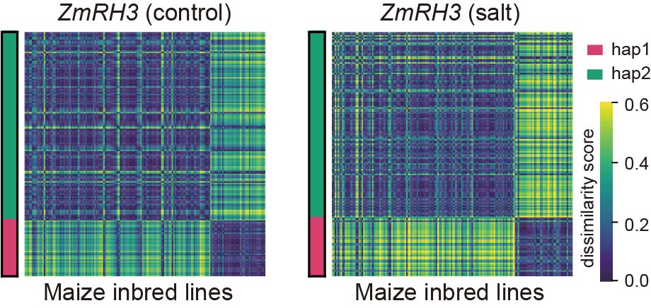
The transformed molecular traits form a distance matrix, and extracting differences from the matrices under stress and control conditions is quite challenging. This involves feature extraction from two matrices and comparison of the differences between features. Contrast PCA is a novel PCA algorithm that can simultaneously process two datasets and automatically extract the most significant differences between them. We used contrast PCA to perform comparison and dimensionality reduction on the transformed molecular traits of the gene ZmRH3. The results showed that in inbred lines with a contrast PCA principal component greater than 0, there was a difference in ZmRH3 expression levels between control and stress conditions; in inbred lines with a principal component less than 0, there was no significant difference in ZmRH3 expression levels between control and stress conditions. This indicates that contrast PCA can be used to extract stress response effects of molecular traits.
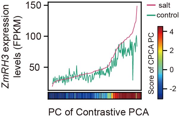
MODAS extracts the stress response effects of molecular traits using the contrast subcommand. This subcommand specifies the omics data under stress and control conditions through the parameters -stress_phe and -control_phe, respectively. It then extracts the stress response effects of molecular traits through Bray-Curtis transformation and the contrast PCA algorithm. The command line is as follows:
MODAS contrast -stress_phe test_salt.rna.phe.csv -control_phe test_control.rna.phe.csv -beta_test_pvalue 1 -o test
Since contrast PCA does not provide statistical significance testing to help screen out insignificant stress response effects, MODAS offers a statistical test method for screening contrast PCA results. The significance threshold is specified through -beta_test_pvalue. The command line including the statistical test screening is as follows:
MODAS contrast -stress_phe test_salt.rna.phe.csv -control_phe test_control.rna.phe.csv -beta_test_pvalue 1e-6 -o test
The above command will generate files with the suffixes .scpca_pc.phe.csv and .scpca_pc.beta_test.csv, which contain the stress response indices of molecular traits and the statistical test results of the stress response indices, respectively.
Note:
It is worth noting that the contrast subcommand by default screens results using Bonferroni multiple hypothesis correction, with a threshold of 1/number of traits tested, and only the stress response effects that pass this threshold are considered as stress response indices.
Identifying stress-responsive molecular QTLs
The stress response index reflects the effects of molecular traits under stress conditions. Performing GWAS on the stress response index can identify molecular QTLs associated with stress response, thereby elucidating the regulatory mechanisms of crop stress tolerance. However, the large number of stress response indices poses a significant computational burden for the identification of molecular QTLs. To address this, we use the MODAS subcommands prescreen and regiongwas to analyze the stress response indices in the process of identifying molecular QTLs related to stress response.
For convenience in simultaneously constructing stress response indices and identifying molecular QTLs, the MODAS subcommand contrast integrates the functionalities of the prescreen and regiongwas subcommands. When using the contrast subcommand to identify molecular QTLs, the parameters -g and -genome_cluster are required to specify the genotype file and the pseudo-genotype file for pre-screening the stress response indices for GWAS analysis.
To analyze the significance of stress response molecular QTLs, we also perform a two-way ANOVA on the identified molecular QTLs. The -anova_pvalue parameter is used to filter the stress-responsive molecular QTLs, yielding the final results. The default threshold for the -anova_pvalue parameter is 0.05. The command line for identifying stress response molecular QTLs is as follows:
MODAS contrast -stress_phe test_salt.rna.phe.csv -control_phe test_control.rna.phe.csv -g chr.TEMs_clump -genome_cluster ./chr.TEMs_clump.genome_cluster.csv -gwas -p 10 -anova_pvalue 0.05 -o test
The above command will generate files with the suffixes .scpca_pc.phe.csv, .scpca_pc.beta_test.csv, .region_gwas_qtl_res.anova.csv, and .region_gwas_qtl_res.anova.sig.csv, which contain the stress response indices of molecular traits, the statistical test results of the stress response indices, the QTL results of the stress response indices including the p-values from the two-way ANOVA, and the QTL results of the stress response indices with significant ANOVA result, respectively.
QTL co-localization analysis based on image matching algorithm
QTL co-localization analysis is a method that integrates multiple phenotypic traits through natural variation, effectively merging various functional information to elucidate the genetic mechanisms of complex traits. However, relying solely on the overlap of QTL regions is insufficient to accurately determine QTL co-localization. The goal of co-localization is to ascertain whether QTLs share the same causal variation, which can be represented through a kinship matrix.
To validate the use of kinship matrices in determining QTL co-localization, we analyzed the stress-responsive metabolite QTL of betaine (SRI1) and the stress-responsive expression QTL of its most relevant candidate gene, ZmGB1. We found that the kinship matrices of both QTLs exhibited a consistent pattern, indicating that kinship matrices can be used to assess QTL co-localization.
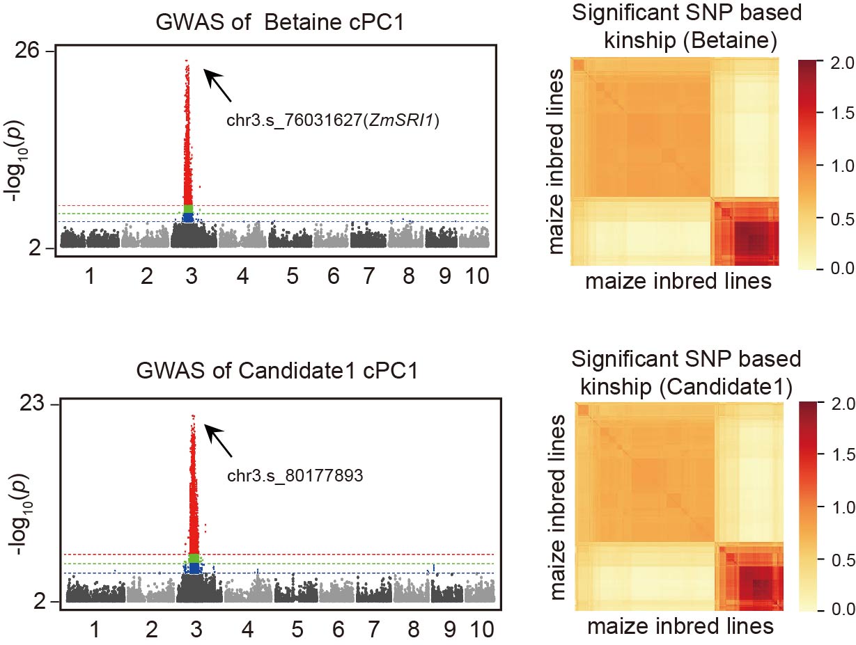
To accurately measure the similarity between two kinship matrices, we used an approximate image matching algorithm. To further evaluate the robustness of this method, we calculated the kinship matrix similarity between the stress-responsive metabolite QTL of betaine (SRI1) and 2666 stress-responsive expression QTLs using the approximate image matching algorithm. The results showed that ZmGB1 had the highest similarity with SRI1, demonstrating that the kinship matrix similarity measure based on the approximate image matching algorithm can be used for QTL co-localization analysis.

MODAS performs QTL co-localization analysis based on the approximate image matching algorithm through the subcommand coloc. The command line is as follows:
MODAS coloc -qtl multi_omics.bc_cspca_res.new.beta_test.sig.region_gwas_qtl_res.anova_sig.csv -g chr.TEMs_clump -gwas_dir gwas_test_new/ -p 8 -o test
The parameter -qtl specifies the QTL file used for co-localization analysis, and -gwas_dir is used to specify the directory containing the association analysis results for each molecular trait. It is recommended to use the association analysis results generated by the MODAS subcommand regiongwas. The parameter -g specifies the genotype data used to calculate kinship, and -p specifies the threads used for co-localization analysis.
The above command will generate files with the suffixes .coloc_res.csv, .coloc_pairwise.csv, and .dis_res.csv, which contain the results of the co-localized QTL clusters, the pairwise QTL co-localization results, and the similarity results between pairwise QTLs, respectively.